Ensemble generation strategies#
NeuroMiner builds ensembles at the CV2 level by combining models learned inside the CV1 folds of a nested, repeated cross‑validation design (see Fig. 9). Version 1.4 adds easy controls for diversity‑aware selection, probabilistic feature extraction (PFE), boosting for both classification and regression, and adaptive wrappers with an automatic stopping rule.
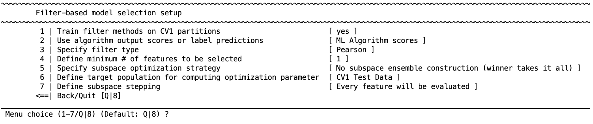
Filter‑based ensemble generalization#
The Subspace Selection Strategy acts as a filter: you rank features, form feature subspaces, train one model per subspace inside CV1, then keep either the single best subspace or an ensemble of the strongest subspaces for CV2 aggregation.
Turn it on#
Menu: Filter‑based model selection setup → Train filter methods on CV1 partitions
Enables the feature‑filtering and subspace workflow.
Prediction type (classification)#
Use algorithm output scores or label predictions
Hard voting (predicted labels)
Soft averaging (probabilities/scores)
(Regression always uses scores.)
Multi‑class ranking (classification)#
Choose binary or multi‑group ranking mode to control how features are ranked across classes.
Evaluation mode#
Choose how ranked features are used:
Subspace mode – build/evaluate blocks of ranked features (e.g., top‑10%, top‑20%, …) and keep one or more subspaces.
Ranking mode – keep the top‑percent of a single ranking (no subspace ensembles).
If you pick Ranking, set the percentile cut‑off (e.g., keep top 5%).
Choose a filter type#
Classification
Mutual information (FEAST) – keeps features that share the most information with the label.
mRMR – balances relevance to the label with low redundancy between features.
Pearson / Spearman correlation – univariate correlation ranking.
SIMBA (margin‑based) – prefers features that widen class margins.
G‑flip (margin‑based) – finds discriminative subsets; option to restrict later steps to features found by G‑flip.
IMRelief (margin‑based) – Relief‑family method with instance‑level weighting.
Increasing feature subspace size – nested subspaces by adding top‑ranked features.
Random subspace sampling – random feature subsets to increase diversity.
Relief (classification) – neighbor‑based margin ranking; set the number of nearest neighbors.
F‑Score (ANOVA) – signal‑to‑noise ratio across classes.
Bhattacharyya distance – class‑distribution separability.
Regression
Mutual information (FEAST)
mRMR
Pearson / Spearman correlation
RGS – regression‑specific ranking.
Increasing feature subspace size
Random subspace sampling
Relief (regression / RReliefF)
Defaults:
• Classification → correlation‑based ranking (Pearson) with subspaces enabled.
• Regression → mRMR.
• Minimum number of features → 1 (you can change this).
Minimum number of features#
Define minimum number of features to be selected
Sets a lower bound for any candidate subspace.
After training subspaces: how to keep models#
Pick one of the following:
Select the single best subspace – “winner takes all”.
Ensemble: keep the top‑X subspaces – you choose X.
Ensemble: keep the top‑percent of subspaces – you choose the percentage.
Ensemble: keep all subspaces.
If you choose an ensemble, configure how to combine the base models:
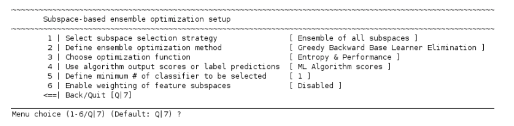
Ensemble optimization methods
Simple averaging — bagging‑style averaging (works with hard or soft predictions).
Backward elimination — start with all models; remove the least helpful ones.
Forward selection — start empty; add the most helpful models.
For 2 & 3, you can optimize by performance, diversity, or both.
Diversity choices include Vote entropy, Double‑fault, Yule’s Q, Fleiss’ Kappa, LoBag error diversity, and (for regression) prediction‑variance/ambiguity.
Optional inverse‑error weighting and minimum number of models to keep.
Probabilistic feature extraction (PFE) — build a consensus feature mask: set an agreement threshold (e.g., “keep features selected in ≥ 75% of high‑performing subspaces”), then retrain one model on that mask.
Boosting — learn weights for the base models to balance accuracy, simplicity, and diversity (see Boosting below).
Target population for the selection criterion — evaluate on CV1 train, CV1 test, or both (recommended: train + test for robustness).
Subspace stepping — define the step size for building cumulative subspaces (e.g., 10% steps → 10%, 20%, 30%, …).
Important
After you have chosen the winning subspaces (or built a consensus mask with PFE), you can hand those features to a wrapper (next section) for deeper, embedded optimization if needed.
Wrapper‑based model selection#
Wrappers search feature combinations that maximize performance inside CV1. You can run them on the full feature set or inside the subspaces created by the filter step.
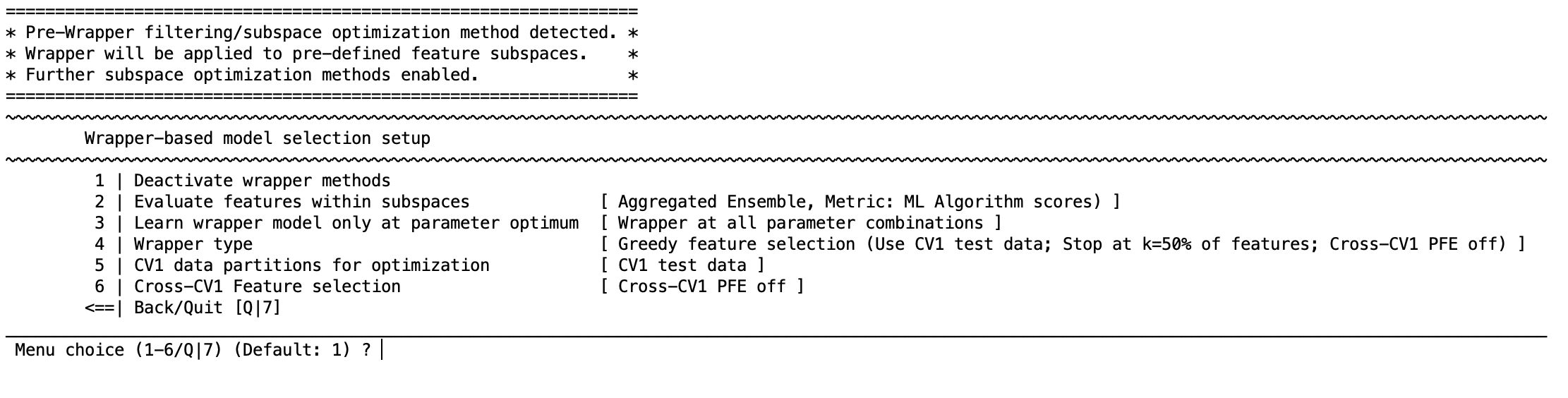
Turn it on & route subspaces#
Activate wrapper methods.
If you previously built subspaces, enable evaluate features within subspaces so the wrapper operates inside each subspace.
Learn wrapper model only at parameter optimum (optional) – if you ran a hyper‑parameter grid, you can limit the wrapper search to the best settings to save time.
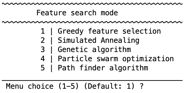
Pick a wrapper & set its options#
Greedy forward/backward selection
Search direction: forward (add) or backward (remove).
Early stopping (optional): stop when a chosen fraction of the pool is reached.
Feature stepping: evaluate one‑by‑one or in small blocks (faster).
Knee‑point threshold (optional): stop where the gain curve flattens.
Simulated annealing
Temperature schedule, cooling, iterations.

Genetic algorithm
Population size, crossover, mutation rate, elites, generations.

Particle swarm optimization
Swarm size, inertia, cognitive/social weights.

Path finder algorithm
Path‑based metaheuristic with an accessible set of knobs.

Data used for wrapper optimization#
Choose whether the wrapper optimizes on CV1 training, CV1 test, both, or the full CV1 partition. Using train + test is usually the safest choice.
Cross‑CV1 feature consolidation (PFE) inside wrappers#
Cross‑CV1 feature selection opens options to keep features that recur across folds:
Agreement with tolerance — “keep features seen in at least p% of folds,” with a fallback tolerance and a minimum number of features.
Top‑N most consistent — select a fixed number from the top of the consistency list.
Top‑percent most consistent — select a fraction (e.g., top 10%).
After selection, choose to retrain each CV1 model after pruning or retrain all CV1 models on the same shared feature set.
New in NM 1.4 — Adaptive wrappers with automatic stopping#
Greedy wrappers no longer depend on an arbitrary “stop at 50%” rule. The adaptive wrapper:
Discourages near‑duplicate features and encourages complementary ones using a smooth, data‑aware penalty.
Stops automatically when further gains fall within the range of normal noise (“natural stopping”).
Works for binary, multi‑class, and regression problems.
What you can control (plain‑English names)
Penalty memory — how quickly past decisions fade.
Baseline drift — a gentle tendency to become more selective over time.
Penalty strength — how strongly redundancy is discouraged.
Encourage‑complementarity zone — where moderately similar features are still considered helpful (you set the center and width).
Near‑duplicate barrier — how forcefully very similar features are penalized.
Smoothness — how gradually the penalty turns on/off.
Stopping sensitivity — a baseline tolerance and a noise factor that decide when improvements are “too small to matter.”
Expert view (optional) — a helper to visualize the penalty curve while tuning.
Tip: Leave these on their defaults to start. They are designed to “do the right thing” without additional tuning. Adjust only if you need tighter or looser selection.
Boosting (classification & regression)#
Boosting learns weights for your base models so the final ensemble balances:
Accuracy — fits the signal,
Simplicity — avoids over‑reliance on any one model,
Diversity — prefers models that disagree in useful ways.
What you can set
Loss type (classification): log‑loss, squared error, or AdaBoost‑style updates.
Diversity strength: how strongly to reward disagreement between models (with an auto‑scale option that picks a reasonable value for you).
Iterations and learning rate (for AdaBoost‑style updates).
Regression diversity choices: measure diversity using residual covariance, residual correlation, or a residual‑graph penalty.
When to use: turn on Boosting if simple averaging underperforms or your subspace models look too similar.
CV2 prediction & aggregation#
After CV1 is complete, NeuroMiner produces predictions in CV2 using an ensemble:
Prediction type
Classification: choose hard voting (majority) or soft averaging (probabilities).
Regression: uses soft averaging.
Retrain on full CV1? Optionally refit the base learners on the entire CV1 partition before CV2 to increase stability.
Aggregate across CV2 permutations
Grand mean — average the CV2 ensemble predictions from each permutation (simple and robust).
Grand ensemble — pool all base learners from all permutations into one larger ensemble (can help when models are diverse).
Shortcut (appears only when nothing needs optimizing): you may be offered to skip the CV1 cycle and train directly on the combined CV1 training+test data. This is disabled automatically whenever an optimization step (filter or wrapper) is active.
Quick‑start presets#
Balanced default (classification)
Filter: correlation ranking → subspaces in 10% steps.
Keep top‑X subspaces with forward selection and performance + diversity.
Use soft averaging at CV2; aggregate by grand mean.
Faster run
Filter: Ranking mode with a top‑5% cut‑off.
Simple averaging of subspace models.
Skip wrappers.
High interpretability
Filter: PFE to build a consensus feature mask.
Train a single model per fold on that mask.
Use soft averaging at CV2.
When accuracy stalls
Turn on Boosting with auto‑scaled diversity, run a few extra iterations, and re‑evaluate.Regression default
Filter: mRMR → subspaces.
Keep top‑percent subspaces, select by performance (optionally add prediction‑variance diversity).
Aggregate by grand mean.