Preprocessing pipeline#
An important part of any machine learning analysis is how the data is prepared or ’preprocessed’ prior to its analysis with a classification algorithm. This is also known as ’feature extraction’ because the features are extracted from the existing data before analysis. NeuroMiner has a number of options to prepare data and can be tailored to a user’s specific data problem.
It’s important to note that NeuroMiner performs preprocessing steps within the cross-validation framework. This means that when the option to preprocess the data is selected, it preprocesses the training data and applies the ’learned’ preprocessing parameters to the CV1 and CV2 test data partitions.
When the preprocessing module is loaded the user will see the following:
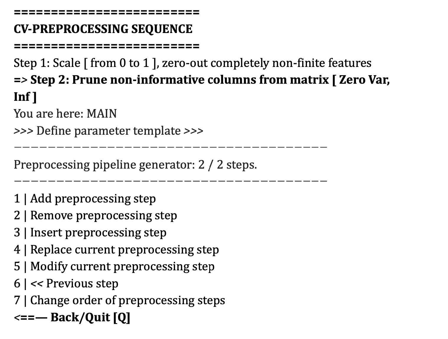
Fig. 10 NeuroMiner preprocessing pipeline setup#
Note
Importantly, the preprocessing steps that are selected will be outlined in order of processing under the heading CV-Preprocessing Sequence. The user can add steps using the add preprocessing step and can modify steps using the other straightforward options within this menu–e.g., the user can modify the settings of a preprocessing step or can change the order of the steps.
Add preprocessing step#
This option is to add a preprocessing step to the ”Preprocessing sequence generator”. Once this is selected, the user can select the option that they would like from the following list:
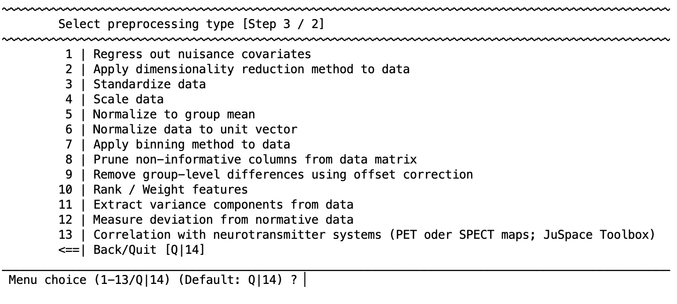
If you are using volumetric neuroimaging data, then there will also be an option included at the top of the list to: 1 | Enable spatial operations using Spatial OP Wizard. This is a special module designed to optimize filtering and smoothing within the cross-validation process and is always performed before any other preprocessing steps across the entire dataset (i.e., on test and training data). Once the user has selected one of the steps, for example to perform a dimensionality reduction, they are redirected to the main preprocessing menu that will add the processing step; for example:
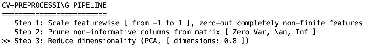
You can see that now there is a line stating CV-PREPROCESSING SEQUENCE containing ”Step 3: Dimensionality reduction”. The ”Preprocessing sequence generator” indicates that the step is selected for further operations as indicated 3/3 (one out of a total of three) steps and this selection is also highlighted by the arrow symbols (>>). If an option requires a suboption (e.g., dimensionality reduction) then the suboption will be listed underneath the parent option and this can be selected using the arrows as well.
As such, you can now perform other operations within this menu, including removing the selected preprocessing step, inserting another preprocessing step at the same location, replacing the current preprocessing step with another one, or modifying the current preprocessing step. If you have added a spatial preprocessing step, then this will appear above this menu because it is conducted prior to the preprocessing sequence across the entire dataset.
Important
The preprocessing steps will be conducted in the order that they appear in the CV-PREPROCESSING SEQUENCE menu.
Enable spatial operations using Spatial OP Wizard#
If your active data modality is neuroimaging data, you should see the following option (see also Fig. 10):
1 | Select spatial operation [ No filtering ]
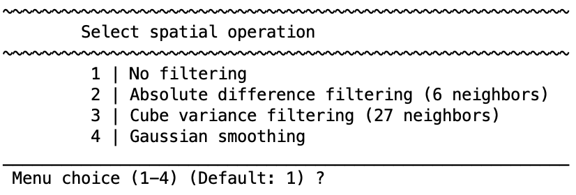
After enabling this mode, you will see the following menu:
Once an option is selected and the parameters have been defined, you will see a new field above the ”CV-PREPROCESSING SEQUENCE” as follows:
Note
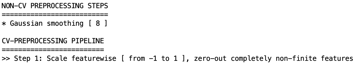
In NeuroMiner, it is designated as ”NON-CV PREPROCESSING” because it occurs across the entire dataset before preprocessing. However, as described below, it’s important to note that for smoothing the user can select a range of parameters and then the optimal combination of smoothing parameters, preprocessing settings, and training settings is found.
2 | Absolute difference filtering (6 neighbors)
Absolute difference filtering is when the difference is computed between the voxel and each of the 6 nearest neighbors surrounding it. Then the value of the voxel is divided by the summed differences of the neighbors.
3 | Cube variance filtering (27 neighbors)
The variance of the 27 neighbors surrounding each voxel is calculated and then the intensity of the target voxel is multiplied by the inverse of this variance.
4 | Gaussian smoothing (=\(>\)FWHM)
This is regular Gaussian smoothing as used in most neuroimaging toolboxes. The advantage of doing this in NeuroMiner is that you can specify multiple different smoothing kernels (e.g., [6 8 10]) and then these will be used as hyperparameters during optimization. That is, during learning in CV1 folds, the best combination of smoothing, other preprocessing steps, and learning parameters will be determined and applied to the held-out CV2 fold.
Regress out nuisance covariates#
If covariates have been entered alongside the data, you can apply covariate correction using this step. This option is designed to remove the variance associated with a nuisance variable (e.g., age, sex, study center) from the data within each CV fold. When chosen it will reveal the following options:
1 | Select method
The first option gives you three possible methods to regress out the covariates: Partial Correlations, ComBat and Disparate Impact Remover (DIR). The partial correlations method computes the coefficients that generate the chosen covariate effects in the data with a general linear model. In addition to the partial correlations method, ComBat also scales the variance estimators. It allows to separate the label (e.g., disease) effects and the covariate effects in the data to some degree. For more detailed information about the ComBat method please check Johnson et al., 2007. Currently, Combat can only be used to correct for batch effects (e.g. site, sex). It requires a numeric vector encoding batch effects to be modeled out. In contrast, partial correlations should be used with a dummy-coded matrix if the user wants to correct for batch effects using this method. Finally, DIR is a method that allows users to transform the features of the dataset so that predictions are fair and do not disproportionately disadvantage any particular group (e.g., race, gender or age groups). Briefly, the algorithm calculates the distribution of values for each selected feature for two or more subject groups (e.g., males and females), calculates the median/mean distribution for all subjects, and applies a percentage of correction (known as repair level, or alpha) to each group towards that median/mean distribution. For a more detailed explanation of the DIR method, please visit the original publication Feldman et al., 2014.
Depending on the selected method, the following configuration options will change. Below there is a description of the options for each method.
Note
Please be aware that ComBat does not provide you with an external validation mode if new sites appear in the test data. For this case, there is a function in NeuroMiner called nk_MultiCentIntensNorm2.m. This function binarizes the interacting covariate and finds the bin with the largest overlap (N) between sites. In this subgroup it computes partial correlation coefficients or offsets and applies those to the entire group to correct for group effects.
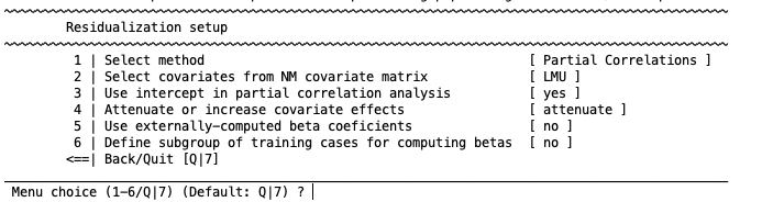
Partial Correlations options#
2 | Select covariates from NM covariate matrix
Selecting the second option will allow you to choose the covariates that you want to control the data with. You select the covariate(s) by entering in either a single numeral (e.g., 1) or many (e.g., 1:2) relating to the covariates that have been previously entered. Once these are selected, the user will be returned to the partial correlations setup menu. Currently, the DIR method only allows for categorical covariates.
3 | Use intercept in partial correlation analysis
The choice of whether to include an intercept is based on your research question and relate to intercept inclusion in any other use of regression.
4 | Attenuate or increase covariate effects
Allows the user to either attenuate or increase the effects of the covariate on the data using regression.
5 | use externally-computed beta coefficients
Allows the user to enter beta coefficients from a regression that has been previously calculated. This option only works if the dimensionality of the beta coefficients exactly matches the dimensionality of the data. This means that NM will crash if the dimensionality of the data is dynamically changed during previous preprocessing steps.
6 | Define subgroup of training cases for computing betas
Option 5 allows the user to define a subgroup of training cases for computing beta coefficients, which are then applied to the data (as discussed in the supplementary material of Koutsouleris et al., 2015 and Dukart et al., 2016). This function is useful when the user does not want to remove variance that may interact with the target of interest. For example, brain volume in schizophrenia interacts with age, therefore, the relationship between age and brain volume can be modeled in the control participants only and then these beta coefficients can be used in the schizophrenia sample to remove the effects of age without removing the effects of illness.
When this option is selected, you will see that another option 7 | Provide index to training cases for computing betas is added to the menu. Select it to define a logical vector consisting of TRUE and FALSE corresponding to the participants in the study; e.g., [0 0 0 0 1 1 1 1]. A FALSE value (i.e., a zero) indicates that they will not be used in the calculation of the betas. A TRUE value (i.e., a 1) indicates that they will be used in the calculation of the betas. Logical vectors can be created from normal double vectors by simply typing ”logical(yourvector)” on the command line (“0”s and “1”s will automatically treated as logical values as well).
ComBat options#
2 | Select covariates from NM covariate matrix
Selecting the second option will allow you to choose the covariates that you want to control the data with. You select the covariate(s) by entering in either a single numeral (e.g., 1) or many (e.g., 1:2) relating to the covariates that have been previously entered. Once these are selected, the user will be returned to the partial correlations setup menu. Currently, the DIR method only allows for categorical covariates.
3 | Retain variance effects during correction
This option allows to retain the variance effects from a selected covariate of interest, while correcting from batch effects from the covariate selected in the option 2. If this option is set to “yes”, a new option will appear: 4 | Define retainment covariates (ComBat method) which allows the user to select the retainment covariate in a analogous fashion to the removed covariate in option 2. Additionally, another option will also be added: 5 | Include NM label in variance retainment. This option allows to include the label (e.g., control vs. schizophrenia) as a retainment covariate. This means that the ComBat algorithm will retain the variance from the different label groups.
6 | Define subgroup of training cases
Option 5 allows the user to define a subgroup of training cases for the ComBat correction, which are then applied to the data (as discussed in the supplementary material of Koutsouleris et al., 2015 and Dukart et al., 2016). This function is useful when the user does not want to remove variance that may interact with the target of interest. For example, brain volume in schizophrenia interacts with age, therefore, the relationship between age and brain volume can be modeled in the control participants only and then the same ComBat correction can be used in the schizophrenia sample to remove the effects of age without removing the effects of illness.
When this option is selected, you will see that another option 7 | Provide index to training cases is added to the menu. Select it to define a logical vector consisting of TRUE and FALSE corresponding to the participants in the study; e.g., [0 0 0 0 1 1 1 1]. A FALSE value (i.e., a zero) indicates that they will not be used in the ComBat calculation. A TRUE value (i.e., a 1) indicates that they will be used in the calculation. Logical vectors can be created from normal double vectors by simply typing ”logical(yourvector)” on the command line (“0”s and “1”s will automatically treated as logical values as well).
Disparate Impact Remover options#
2 | Select covariates from NM covariate matrix
Selecting the second option will allow you to choose the covariates that you want to control the data with. You select the covariate(s) by entering in either a single numeral (e.g., 1) or many (e.g., 1:2) relating to the covariates that have been previously entered. Once these are selected, the user will be returned to the partial correlations setup menu. Currently, the DIR method only allows for categorical covariates.
3 | Type of distribution
Measure used to calculate the “ideal” feature distribution used for correction. If the mean is selected, then the ideal distribution is calculated by calculating the mean of frequency of each bin among all the distributions from the covariate groups. If the median is selected, the same process is applied, but using the median.
4 | Strength of correction
This option determines the repair level. A value of 0 will apply no correction (the feature distribution will remain the same), while a strength of correction of 1 will totally correct the distributions to the mean/median distribution among the covariate groups.
5 | Define subgroup of training cases
Option 5 allows the user to define a subgroup of training cases for computing the DIR distributions, which are then applied to the data (as discussed in the supplementary material of Koutsouleris et al., 2015 and Dukart et al., 2016). This function is useful when the user does not want to remove variance that may interact with the target of interest.
When this option is selected, you will see that another option 6 | Provide index to training cases is added to the menu. Select it to define a logical vector consisting of TRUE and FALSE corresponding to the participants in the study; e.g., [0 0 0 0 1 1 1 1]. A FALSE value (i.e., a zero) indicates that they will not be used in the calculation of the distributions. A TRUE value (i.e., a 1) indicates that they will be used in the calculation. Logical vectors can be created from normal double vectors by simply typing ”logical(yourvector)” on the command line (“0”s and “1”s will automatically treated as logical values as well).
Apply dimensionality reduction method to data#
A common need in machine learning analysis is to reduce the dimensionality of the data within the cross-validation framework (e.g., with structural neuroimages containing about 50,000 voxels). NeuroMiner allows the user to do this using a number of different methods. When the option to reduce dimensionality is selected, the user will be shown the following menu:
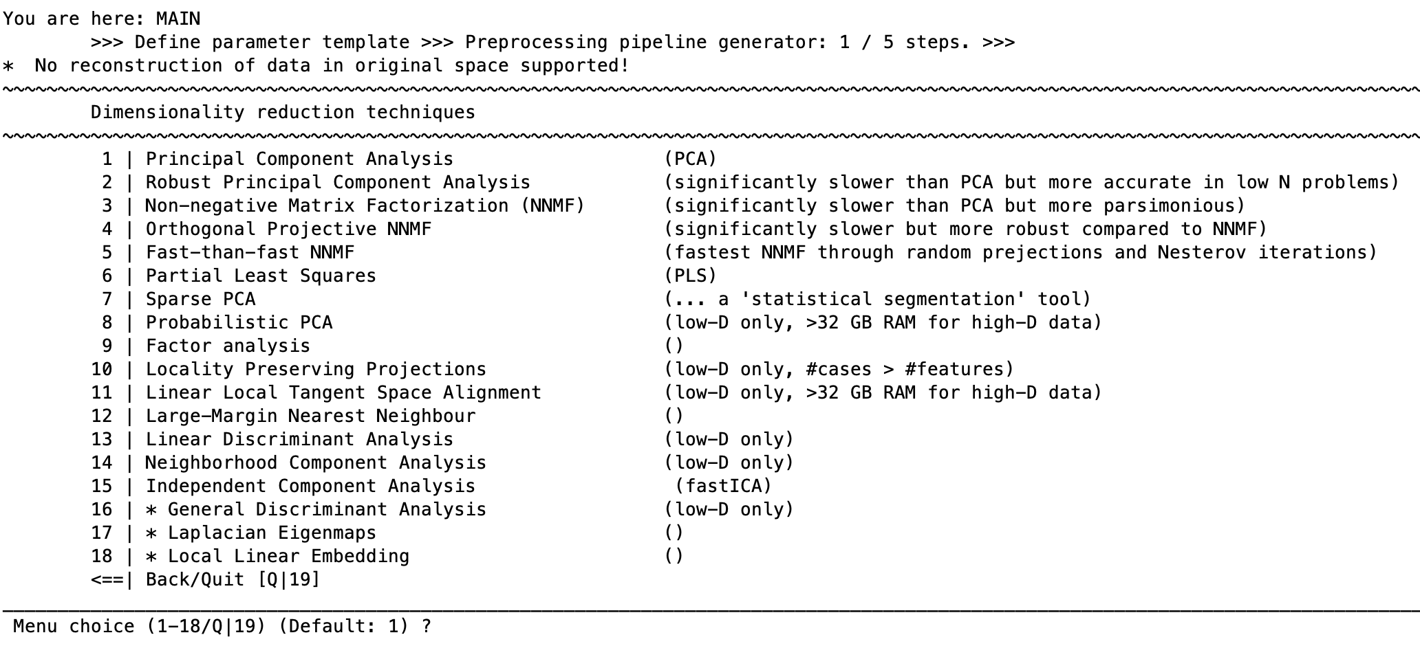
Each of these options will ask for parameters that are specific to the type of dimensionality reduction being conducted and are included in the respective sites for each technique listed below.
The main variable that can be changed across dimensionality reduction types is the number of dimensions that are retained following reduction (e.g., retaining 10 PCA components following dimensionality reduction of neuroimaging data). The following example applies to PCA reduction because this is the most common and we have found that it produces robust results.
For PCA, NeuroMiner gives the option to select the number of dimensions with the following options:
1 | Define extraction mode for PCA [ Energy range ] 2 | Define extraction range [ 0.8 ]
These options allow the user to select how the components are extracted and an extraction range based on this setting. When option 1 is selected, you will see the following menu:
1 | Absolute number range [ 1 … n ] of eigenvectors 2 | Percentage range [ 0 … 1 ] of max dimensionality 3 | Energy range [ 0 … 1 ] of maximum decomposition
1 | Absolute number range [ 1 … n ] of eigenvectors: A whole number of components that they would like to retain a priori.
2 | Percentage range [ 0 … 1 ] of max dimensionality: A percentage of components to keep out of the total number of components.
3 | Energy range [ 0 … 1 ] of maximum decomposition: Retaining components based on the percentage of the total amount of variance explained (i.e., energy). For example, you might want to keep all components that explain 80% of the variance of your data.
For each of these options, except PLS, NeuroMiner gives the user the option to optimize the number of components that are selected during cross-validation by specifying a range of values. For example, a range of 20%, 40%, and 60% can be selected by entering [0.2 0.4 0.6]. NeuroMiner will then conduct all optimization procedures using these percentages of retained variance–i.e., it will find the best PCA reduction considering the other settings. If a range of values is required, then it is recommended that an additional substep is performed.
Extracting Subspaces#
NeuroMiner has an additional option to first conduct the decomposition and then to retain different component numbers for further analysis. You do this by following the above procedure, but specifying that you want to retain a singular value of components (e.g., for PCA, 100% of the energy is recommended for the next step). Then you return to the preprocessing menu and select the option to ”Add a preprocessing step”. In the list of steps, there will now be an option to ”Extract subspaces from reduced data projections” and the following menu will appear:
1 | Define extraction mode for PCA [ Energy range ] 2 | Define extraction range [ 1 ]
Using these functions you can then select the components that you want to retain without having to run separate dimensionality reduction analyses. For example, you can retain 100% of the energy in the first step of a PCA to reduce the data dimensions and then retain a range of subspaces of components in the second step; e.g., [0.2 0.4 0.6 0.8]. This drastically increases processing time. The following advanced dimensionality reduction techniques are also offered by NeuroMiner, and the settings will change based on the technique. We recommend to follow the links provided below to determine the settings that are required or to evaluate the default settings offered within NeuroMiner.
Dimensionality Reduction Techniques
Principal Component Analysis (PCA) - PCA by Deng Cai
Robust Principal Component Analysis - LIBRA
Note that RPCA is significantly slower than PCA but more accurate in low N problems.Non-negative Matrix Factorization - Li and Ngom’s NMF toolbox
Note that NMF is significantly slower than PCA but more parsimonious & robust.Partial Least Squares performs a single value decomposition (SVD; matlab built-in) on a covariance matrix constructed from the entered features plus another feature set to get latent variables. For example, if the primary features are voxels from a brain and the secondary PLS feature set are the labels it conducts SVD on the combined matrix (after standardization). It then multiplies this unitary matrix (U) from the SVD with the original standardized primary feature matrix in order to sensitize the analysis to the combination of the features. Other data can be used in place of the labels. The user has the option to use sparse PLS based on the function ”spls”.
Sparse PCA - [Please check preproc/spca.m; Zou et al., 2004] This is a ‘statistical segmentation’ tool.
Simple Principal Component Analysis - MTDR; van der Maaten
Probabilistic PCA - MTDR; van der Maaten This option is only for low dimensional problems, it requires more than 32GB RAM for high-D data.
Factor analysis - MTDR; van der Maaten
Locality Preserving Projections - MTDR; van der Maaten This option is only for low-dimensional problems. Number of cases needs to be greater than the number of features.
Linear Local Tangent Space Alignment - MTDR; van der Maaten For low-D only, requires >32 GB RAM for high-D data.
Large-Margin Nearest Neighbour - MTDR; van der Maaten
Deep Autoencoder – MTDR; van der Maaten Low dimensional data only.
Neighborhood Component Analysis MTDR; van der Maaten This option is only for low-dimensional problems.
fastICA - fastICA, sklearn function, fastICA, publications, A. Hyvärinen
Orthogonal Projective Non-Negative Matrix Factorization - GitHub, Paper
For an overview and the implementation of all techniques see nk_PerfRedObj.m and files in the preproc directory.
Standardize data#
The standardization, scaling, and/or normalization of data is an important part of most machine learning. NeuroMiner contains different methods to perform these functions within the preprocessing modules, which are conducted within each inner cross-validation fold. Standardization is conducted on each of the features that have been entered to NeuroMiner across observations.
When option “3” is selected, the user will see the following:
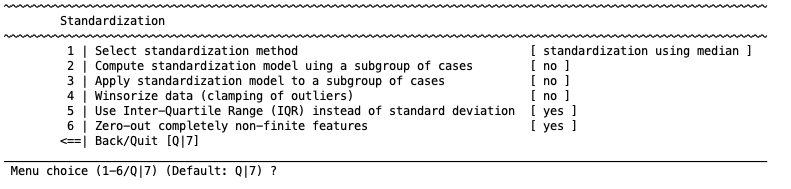
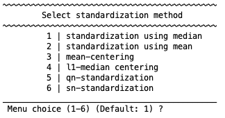
1 | Select standardization method
Select from the following standardization options:
Note
calculates the Z-score using the median (i.e., (score -median) / standard deviation / interquartile range).
calculates the Z-score using the mean.
mean-centers all features (i.e., subtraction of the mean for the feature across all scores).
calculates the multivariate L1-median and then takes the derivatives from this as features (see nk_PerfStandardizeObj.m; Hossjer and Crous (1995).
and 6. are alternatives to the median absolute deviation for standardizing multivariate data (see Rousseeuw and Croux (1993)).
2 | Compute standardization using a subgroup of cases
User can compute the standardization using a subgroup of cases.
3 | Apply standardization model to a subgroup of cases
User can apply the standardization model to a subgroup of cases.
4 | Winsorize data (clamping of outliers)
The user also has the option to Winsorize or ’censor’ the data. This technique was introduced to account for outliers. After standardization, the elements which are outside of a user-defined range (e.g., 4 standard deviations) are set to their closest percentile. For example, data above the 95th percentile is set to the value of the 95th percentile. The feature is then re-centered using the new censored values.
5 | Zero-out completely non-finite features
If there are entries in the user’s feature data that are non-numeric (i.e., ”NaN” or ”not a number” elements), then these will not be considered during the calculation of the mean and standard deviation (NeuroMiner uses the nanmean function). However, after the data has been standardized, these values will be added back to the feature matrix. As such, NeuroMiner gives the option to change these to zero in step four. It is important to note that once the data has been standardized, zero values reflect the mean of the feature and are thus a form of mean imputation. If the user wants to use other imputation options, they can select ’no’ to this option and then impute the data using the preprocessing imputation option.
Scale data#
Another option to put the data into the same space is to scale it between two values. The user will see the following menu when they select this option:
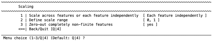
1 | Scale across features or each feature independently [each feature independently]
Here you have the choice between scaling ”each feature independently” or ”across the entire matrix”. If each feature independently is selected, then the data will be scaled within the desired range for each feature (i.e., each voxel or each questionnaire). If the entire matrix is selected then each value in the matrix will be scaled according to the range of all the data (e.g., all voxels or all questionnaires).
2 | Define scale range [0,1]
The user then has the option to define the scale range between 0 and 1 or between -1 to 1. These two chices are provided because some machine learning algorithms require the data to be scaled differently; e.g., the LIBLINEAR options require the data to be scaled between -1 to 1.
Important
Make sure to check whether the algorithm of your choice requires a certain scale!
3 | Zero-out completely non-finite features [yes]
Non-numeric values are not taken into account during scaling and are added back to the matrix after scaling. The third option gives the user the ability to either change these values to zero following scaling by selecting ”yes” for the third option to ”zero-out completely non-finite features”. It is critical to note that in this case the values will be considered to be the absolute minimum of the scale for future analyses (e.g., if IQ is scaled, then these individuals will have an IQ value of 0).
Tip
For questionnaire data, it is recommended that this option is changed to ”no”, and instead imputation is performed for the NaN elements after scaling. Alternatively, for imaging data, it is recommended that NaN values are excluded by using a brainmask during data input. Furthermore, starting with NM 1.1, zero-variance columns encountered by the scaling function will be automatically set to zero instead of NaN. This allows for their subsequent removal using the pruning module, prior to e.g. imputation.
Normalize to group mean#
This option is only available when a group has been entered as a covariate at the start of the analysis (i.e., dummy coded vector containing ones for the group and zeros for the other participants). The option will then normalize all subjects to the mean of the specified group.
Normalize to unit vector#
This option takes the mean of the data, then subtracts this from each of the scores within the data. It then calculates the norm (L1 or L2) of this result. It then mean-centers the original data and divides each score by the normalized scores.
Apply binning method to data#
Binning is a technique that can be used to control for variance in data (wiki). For example, a histogram is an example of data binning. A form of it is discretization of continuous features (wiki) and this is offered in NeuroMiner as the default option when binning is selected as follows:
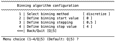
Discretization basically just forms bins based on the standard deviation. You first establish a vector using a start value, a stepping value, and a stop value called alpha (e.g., the default setting is [0 0.5 1 1.5 2 2.5 3 3.5 4]). It then discretizes each feature by the mean +/- alpha*std. For example, for the first value of alpha, it finds the feature values that are above and below the mean and gives them a new value (i.e., 1 or -1). Then in the next step it finds the values that are above and below the mean +/- half of the standard deviation and gives them a new value (i.e., 2 or -2). In the next step it finds values that are above and below one standard deviation from the mean and gives them a new value (i.e., 3 or -3). And so on. In this way, bins are created with a width that is determined by the standard deviation.
Note
It is important to note that this function will perform Winsorization (i.e., clamping) because values above the stop value of alpha (e.g., above 4 standard deviations above or below the mean) will be clamped to the user-defined alpha value (e.g. 4) .
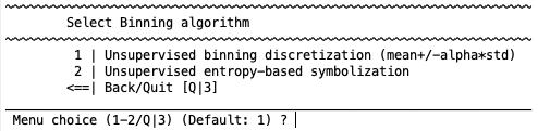
Manually determining the bins is a good way to discretize data if you have a firm idea about the problem, but if you do not then it is useful to find an optimal bin width for a feature by taking into account the information content of the data. This can be done in NeuroMiner by changing the ”1: Select binning method” to ”Unsupervised entropy-based symbolization”. It tries to find an optimal bin width for a feature by taking into account the entropy. It will do this within the range that you specify in the following settings:
Impute missing values#
Note
NeuroMiner will only show this preprocessing option in the list in case there are NaN values in your data!
The machine learning algorithms included in NeuroMiner are not able to process missing values (represented in MATLAB as ”Not a Number” (NaN) entries). This means that they have to be either removed using the ”Prune non-informative columns” feature described below, or they need to be imputed using this module. NeuroMiner performs imputation using either single-subject median replacement, feature-wise mean replacement, or multivariate distance-based nearest neighbor median imputation. When this feature is selected it will reveal the following menu:
1 | Define imputation method [ kNN imputation (EUCLIDEAN) ]
2 | Select features for imputation [ All features ]
3 | Define number of nearest neighbors [ 7 nearest neighbors ]
1 | Define imputation method#
You have to first define the imputation method using the following menu:
1 | Median of non-NaN values in given case
2 | Mean of non-NaN values in given feature
3 | MANHATTAN distance-based nearest-neighbor search
4 | EUCLIDEAN distance-based nearest-neighbor search
5 | Sequential kNN-based imputation method (EUCLIDEAN)
6 | SEUCLIDEAN distance-based nearest-neighbor search
7 | COSINE similarity-based nearest-neighbor search
8 | HAMMING distance-based nearest-neighbor search
9 | JACCARD distance-based nearest-neighbor search
10 | Nearest-neighbor imputation using hybrid method
For median or mean replacement, values are imputed based on the data either across features for one subject or across subjects within the feature. For multivariate nearest-neighbor imputation, for each case with NaN values, a multivariate statistical technique is conducted to identify a number of similar (i.e., nearest-neighbor) cases from all the subjects that are available. For example, the Euclidean distance could be used to identify the 7 nearest-neighbor subjects that are close to the subject with the NaN value. Once these similar cases are identified in the multivariate space, then NeuroMiner will take the median of their values of the feature with the missing NaN case and impute it into the NaN field. A number of distance metrics can be used to represent the cases in multivariate space and to determine the nearest-neighbors based on the type of data you have (e.g., Manhattan, Euclidean, Seuclidean, Cosine, Hamming, or Jaccard). For example, the Euclidean distance could be used for data with a continuous measurement scale or the Hamming could be used for binary nominal data (i.e., 0 or 1) data (see Nominal Data). There is also the option to use a hybrid approach that accounts for both continuous/ordinal and nominal data. It’s important to note that all options require the Statistics and Machine Learning Toolbox of MATLAB.
Median of non-NaN values in given case
This function checks NaN values for each subject. When it finds a NaN value for a subject, it imputes the median of the non-NaN values across the other features for that subject. Therefore, this would make no sense at all if it was done across features that weren’t equivalent in scale or from the same scale (e.g., a questionnaire). As such, it could be used in combination with the option to “2 | Select features for imputation” described below.
Mean of non-NaN values in given feature
This function cycles through each feature and if it finds a NaN value then it imputes the mean of non-NaN values.
MANHATTAN distance-based nearest-neighbor search
This function determines the Manhattan distance between cases and then selects nearest-neighbors. You must scale, unit-normalize or standardize the data first, otherwise the distance measure will be dominated by high-variance features.
EUCLIDEAN distance-based nearest-neighbor search
Determines the Euclidean distance between cases and then selects nearest-neighbors. You must scale, unit-normalize or standardize the data first, otherwise the distance measure will be dominated by high-variance features.
Sequential kNN-based imputation method (EUCLIDEAN)
Faster than previous option.
SEUCLIDEAN distance-based nearest-neighbor search
The Seuclidean distance between cases is measured using the pdist2 function that is built into the Statistics and Machine Learning Toolbox of MATLAB.
COSINE similarity-based nearest-neighbor search
The Cosine distance between cases is measured using the pdist2 function that is built into the Statistics and Machine Learning Toolbox of MATLAB.
HAMMING distance-based nearest-neighbor search
The Hamming distance between cases can be used for nominal data (e.g., 0/1 data) and is measured using the pdist2 function that is built into the Statistics and Machine Learning Toolbox of MATLAB.
JACCARD distance-based nearest-neighbor search
The Jaccard distance between cases is measured using the pdist2 function that is built into the Statistics and Machine Learning Toolbox of MATLAB.
Nearest-neighbor imputation using hybrid method
This option combines techniques that can be used for binary nominal data (i.e., 0/1) and ordinal/continuous data. You must define a method for nominal features (e.g., Hamming or Jaccard) and then define a method for ordinal/continuous features (e.g., Euclidean or Cosine). The maximum number of unique values for nominal feature imputation must also be specified.
Nominal Data
It is important to remember that nominal data with more than two categories needs to be dummy-coded for the results to make sense (i.e., 0 or 1 coding). NeuroMiner does not recognize the types of a variable and therefore nominal data that is coded with more than three categories (e.g., 1=Depression; 2=Bipolar; 3=Schizophrenia) will be modeled as a variable with meaningful relationships between the numbers when differences are actually arbitrary.
2 | Select features for imputation#
The imputation procedures can be applied to the entire dataset or to subsets of the data. This is useful when there are different data domains (e.g., clinical and cognitive data) or even single questionnaires (e.g., the PANSS) that you want to restrict the imputation to. A MATLAB logical vector (i.e., consisting of TRUE and FALSE fields that are depicted as [0 0 0 1 1 0 0 etc.]; you can convert a binary vector to a logical simply by typing logical(yourvector) on the command line) must be provided to select a subset. If you want to impute multiple subsets then you must add separate imputation routines. Please note: If previous preprocessing operations change the dimensionality of the feature space (e.g. pruning) these changes are propagated to the user-provided logical feature indices used by the imputation module.
Note
If previous preprocessing operations change the dimensionality of the feature space (e.g. pruning) these changes are propagated to the user-provided logical feature indices used by the imputation module.
3 | Define number of nearest-neighbors#
If you’re using the multivariate nearest-neighbors approach then you must define the number of nearest neighbors (e.g., subjects) to use for the calculation of the median value. The default is 7.
Caution
We found that this step yields stable results when data is scaled prior to the imputation step, however the results become unstable when the data is standardized.
Prune non-informative columns from data matrix#
Data pruning is the removal of examples or features that will not work with machine learning algorithms or are redundant. In NeuroMiner, the machine learning algorithms that are used cannot work with missing values (i.e., ”Not a Number” (NaN) entries in MATLAB) or with infinite values (i.e., ”Inf” in MATLAB), which can occur due to previous processing steps. If the values of a feature do not change between participants (i.e., there is zero variance), then it is redundant to include the feature in the analysis as well. To correct for these problems, NeuroMiner offers the following options:
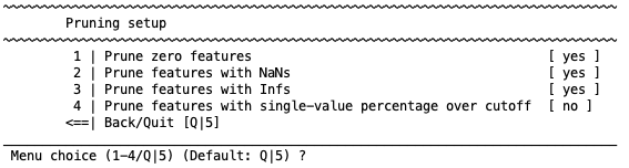
1 | Prune zero features [ no ]
The first option gives the user the ability to remove variables with no variance within a fold (i.e., if all individuals, or ’examples’ within a cross-validation fold have exactly the same value for a feature).
2 | Prune features with NaNs [ yes ]
The second option will remove features within a fold that have any NaN (’Not a Number’) values.
3 | Prune features with Infs [ yes ]
Similarly, the third option will allow users to remove features with any Infs (Infinity) values.
Important
Be careful with pruning! Even if there is one subject with one NaN or Inf within the fold NeuroMiner will remove the feature. The amount of removed features will be difficult to quantify. For matrix data, check the NaNs and potentially filter them prior to the entry into NeuroMiner (see Fig. 4).
4 | Prune features with single-value percentage over cutoff [ yes, 5 ]
The fourth option is used in situations where there are a large number of subjects with the same value and a few with different values. For example, in neuroimaging due to registration inaccuracies most of the subjects may have a voxel value of zero in a location close to the gray matter border and a few might have non-zero numbers. In these circumstances, you might want to exclude the voxels where there is no variance in, for example, 90% of the sample (e.g., where 90% of individuals have a zero value). You can specify a percentage here to do this.
Remove group-level differences using offset correction#
This function was introduced primarily to control for scanner differences in structural neuroimaging data. In the case of two centers, for each feature, the mean of both center A and center B is calculated. The mean difference between these is then calculated (A-B=Y) and then subtracted from each of the data points in A (i.e., Ai - Y). This value is stored for further analysis. Internal empirical tests indicate that this simple method can effectively control for major site differences.
Rank / Weight features#
Selecting or ranking features is an important part of machine learning and can be achieved with filters and wrappers. For a discussion of why these methods are important and for all definitions see Guyon et al., 2003.
Note
Wrappers and will further be discussed in ensemble generation straqtegies.
Filter methods broadly involve the weighting and ranking of variables, and optionally the selection of top performing variables. This can be conducted either prior to the evaluation of the model during pre-processing or as part of model optimisation (discussed in section ensemble generation straqtegies). This option allows the user to weight variables in the training folds based on some criteria (e.g., Pearson’s correlation coefficient with the target variable) and then rank them in a specified order (e.g., descending order from most to least correlated). When this option is selected, the following will be displayed:
1 | Choose algorithm and specify its parameters
The user here has the option to choose from among a number of methods that will weight the relationship between the filter target and the feature. These are:
Pearson / Spearman correlation: Standard MATLAB functions for Pearson’s (corrcoef.m).
Spearman correlation: Standard MATLAB function for Spearman’s (corr.m).
G-flip (Greedy Feature Flip): See Gilad-Bachrach et al. (2004) and site
Simba: See Gilad-Bachrach et al. (2004) and link
IMRelief: This is an implementation of the Yijun Sun IMRelief function called “IMRelief Sigmoid FastImplentation” (see Sun & Li, 2007).
Relief for classification: This is a version of the built-in MATLAB ReliefF algorithm (link).
Linear SVC (LIBSVM): This weights the features by conducting a linear SVM using each independent feature, as implemented in LIBSVM (Chang & Lin).
Linear SVC (LIBLINEAR): Weights the features based on using LIBLINEAR toolbox (link)
F-Score: Weights the features based on conducting an ANOVA using standard MATLAB functions on the differences between the groups when problem is classification.
AUC: Calculates an area under the curve (AUC) for binary classifications based on the code of Chih-Jen Lin (Lin, 2008)and then ranks the features based on this.
FEAST: Implementation of the FEAST toolbox for feature selection (site).
ANOVA: Standard implementation of ANOVA.
PLS: Performs a Partial Least Squares analysis to rank the features.
External ranking: This option uses a user-defined weighting template that was entered during [data input] (input_data), to use an external weighting map from a file, or to read-in a weighting vector using the MATLAB workspace.
2 | Define target labels Here the user defines the target label that the filter will be applied to using the original data; e.g., this could be your group labels if you have a classification problem or your questionnaire item if you’re using regression. The default setting in NeuroMiner is to use your target variable, but this can be changed by first selecting the menu item and then entering ”D” to define a new target label. A new menu will appear and you can select to enter either categorical or continuous data. You can then enter a MATLAB vector that defines either categorical labels (e.g., [0 0 0 0 1 1 1 1]) or continuous labels (e.g., [15 26 19 33 22]). These variables should be stored in your MATLAB workspace. When a continuous variable is selected, the user will then be asked whether they want to weight feature using only one specific subgroup. This means that the feature will only be weighted only based on the relationship between the feature and the filter target in one subgroup (e.g., control participants).
3 | Up- or down-weight predictive features This option allows the user to either upweight or downweight the features based on the relationship between the variable and the target. For example, if you want to increase the importance of the features based on the target you would upweight the features. If you want to reduce the importance of the fea tures based on some other variable (e.g., age if it is a nuisance variable) you could select the variable as the feature selection target and then choose the downweight option. For more information about why you would want to do this see references above.
Extract variance components from data#
This function takes a source matrix and performs a PCA. It then determines correlations between the eigenvariates from the PCA reduction, and those above or below a specified threshold are identified. It then projects the target matrix to the source matrix PCA space, and then back-reconstructs this to the original input space without the identified PCA components (i.e., it removes the variance associated with those components).
Measure deviation from normative data#
This function calculates a partial least squares (PLS) model and then determines how much the data deviates from the model that is produced. The hypothesis here is that the PLS model represents a normative variation between the primary features (i.e., your (processed by previous preprocessing steps in your pipeline) features which were entered into NM, e.g., brain data) and the second feature matrix which you can load into NM when setting up this step (e.g., covariates, like age and/or sex).
How does it work? PLS first extracts a set of latent factors that explain as much of the covariance as possible between the primary features and the covariate matrix. Next, a regression predicts values of the primary features using the decomposition of the covariates.
Finally, the normative deviation is computed (primary features - predicted primary feautures) and replaces the primary features in further processing steps.
Warning
The outcome label should not be entered in the covariate matrix since the information will otherwise be introduced into the processed feature data and, therefore, inflate performance.
Regression mode: Target scaling & transformation#
In the regression setting, one has the option to enable scaling of the outcome variable (default). Further, a number of transformations for the outcome variable are available as well.