Result Viewer#
Once initialization, preprocessing, and model training have been performed, the results can then be viewed using this option. The results display interface can be understood in three main divisions:
the accuracy and model performance (initial screen)
the model performance across the selected hyperparameters
results concerning the individual features in the analysis
Accuracy and model performance#
See {numref}(fig:Display_ClassPlot): The performance of a model can be fundamentally described by the degree to which the predictions match the target scores (e.g., how many people are classified correctly or how closely the features and target are related in a regression). In NeuroMiner, this is represented in multiple ways that each address a different aspect of the relationship between subjects, predictions, and targets.
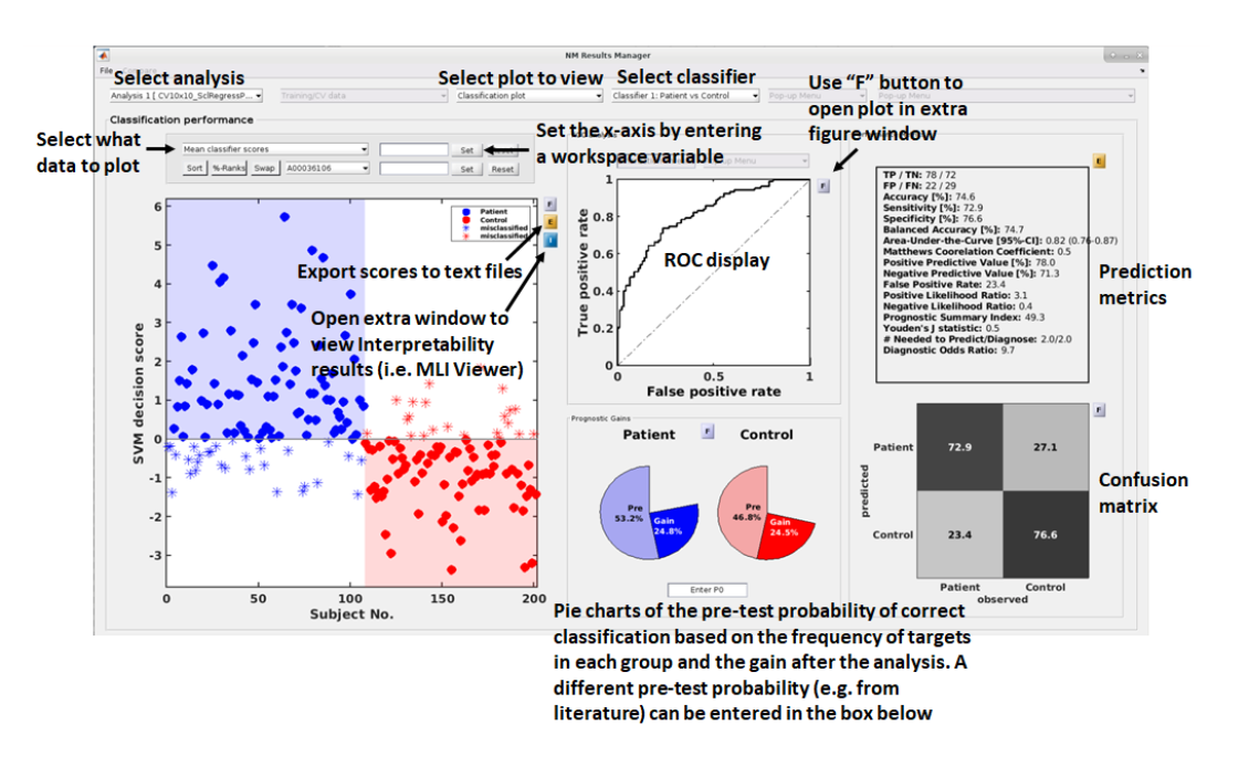
Fig. 12 Result viewer option 1: Classification plot#
Model comparisons#
The user can perform statistical or visual comparisons when there is more than one analysis:
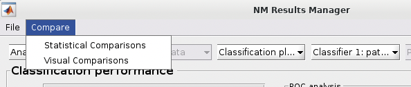
See {numref}(fig:NM_resultviewer_statistical_comparison): Statistical comparisons can be conducted between the model performances using a variety of statistics using the ”Statistical Comparisons” option. The results of these comparisons are output in either excel spreadsheet files (i.e., xlsx) or in text files (i.e., csv) for Linux and Mac. The menu is quite intuitive (i.e., as below) where you select the analyses you want to compare on the right, you press the ”Save As” button to choose a name, and then you select the ”Compare” button to generate the files. The files will be generated in your working directory.
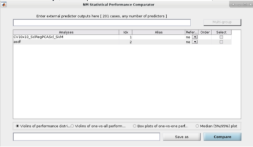
Fig. 13 Within the main results display, the user can go to the ”Comparisons” menu item and then select the option to calculate statistical differences between separate models#
See Fig. 14: The user can also perform ”Visual Comparisons”. The user needs to select some performance measures that they want to compare visually in the top-half of the pop-up box using the ”Select” column tick-boxes, then select the analyses in the lower-half of the pop-up box. Then simply press ”Visualize”. If the bar plots are not good then the user can change it to ”Line plots” and then press ”Visualize” again.
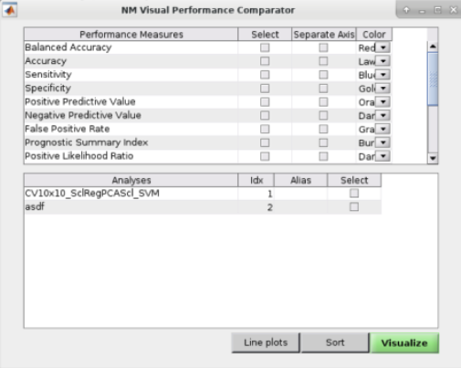
Fig. 14 Within the main results display, the user can go to the ”Comparisons” menu item and then select the option to display visual comparisons between separate models#
Note
Due to incompatibilities of MATLAB’s App Designer with MATLAB versions older than R2021a, this model comparison tool only works in MATLAB R2021a and newer versions.
Classification performance#
See Fig. 15: NeuroMiner was built to work with hyperparameter optimization within a nested-cross validation framework as a standard. In this plot, you will see the inner-cycle, CV1, mean test performance plotted in blue and then the outer cycle, CV2, mean test performance plotted in red. Each point represents a hyperparameter combination. This gives an indication of how the hyperparameter combinations are influencing the test performance. On the right, the display also shows heatmaps that show how the performance in the CV1/CV2 folds changes over the permutations.
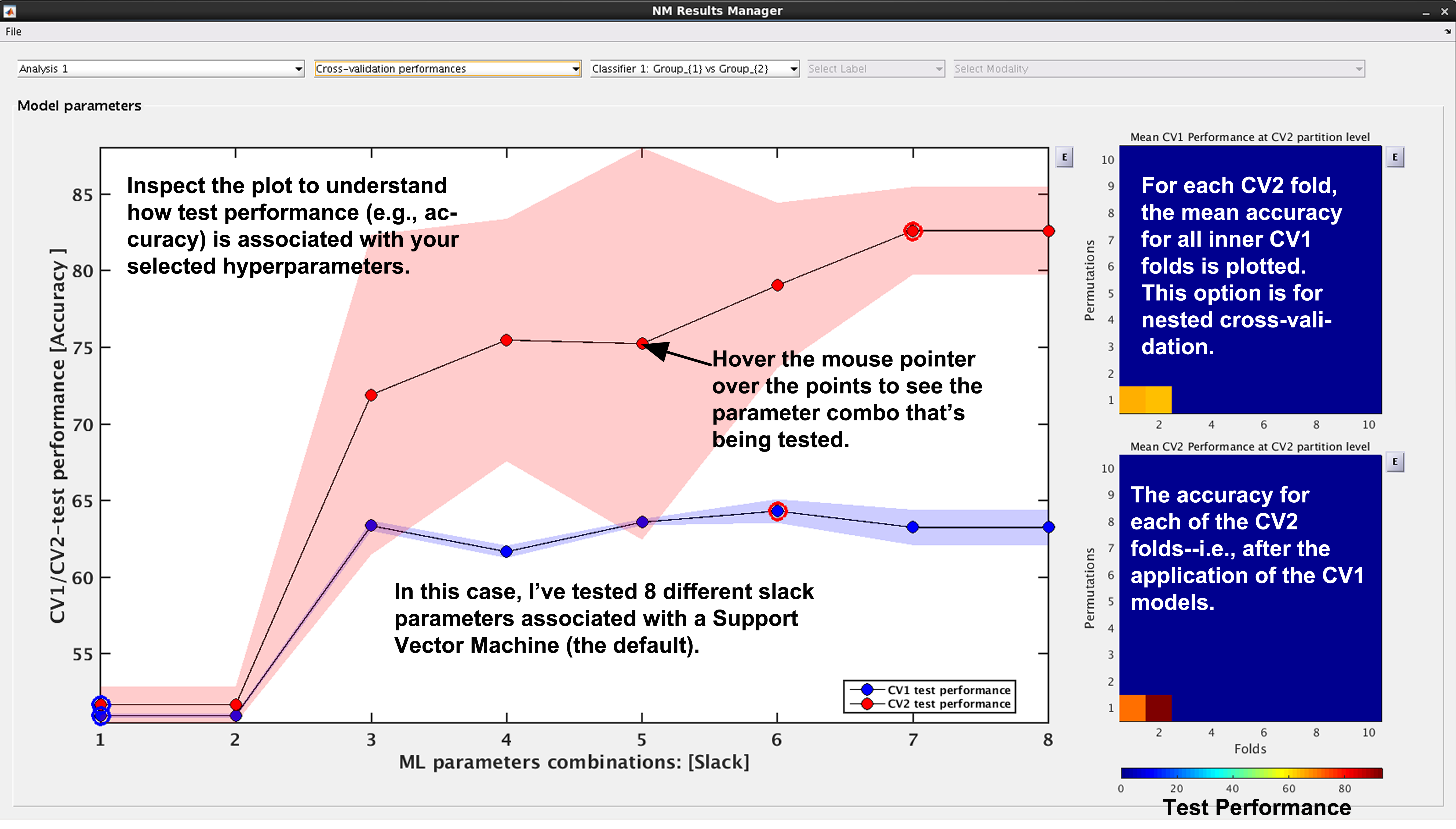
Fig. 15 Result viewer: Cross-validation performance#
Generalization error#
See Fig. 16: Another way to look at CV2 test performance is with the generalization error, which is calculated in NeuroMiner as the CV1-test performance minus the CV2 test performance.
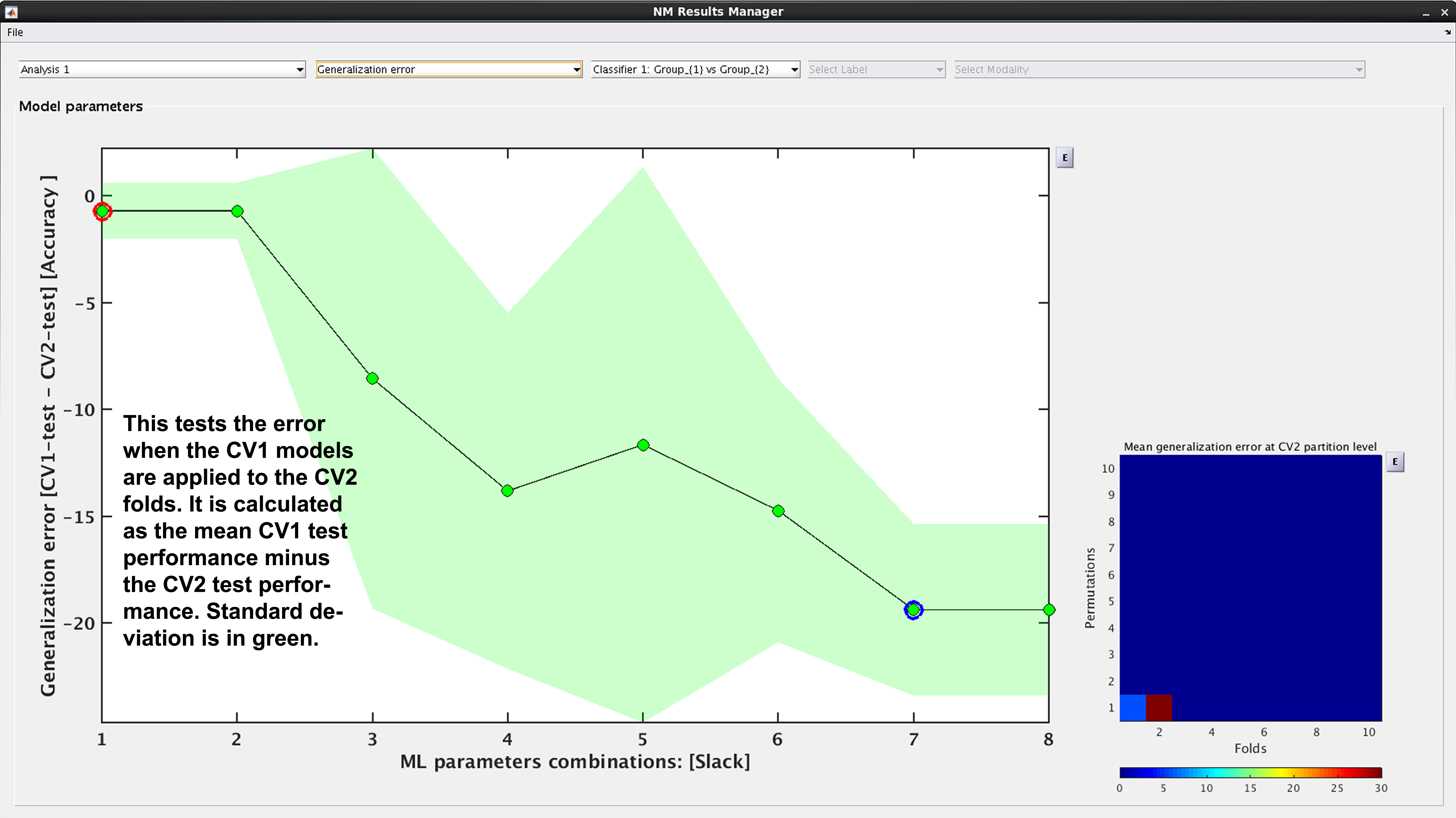
Fig. 16 Result viewer: Generalization error#
Model complexity#
See Fig. 17. In NeuroMiner, complexity is defined as the percentage of support vectors divided by the number of subjects in the tested fold. This feature is useful to determine how varying parameter combinations may affect the fit of the model.
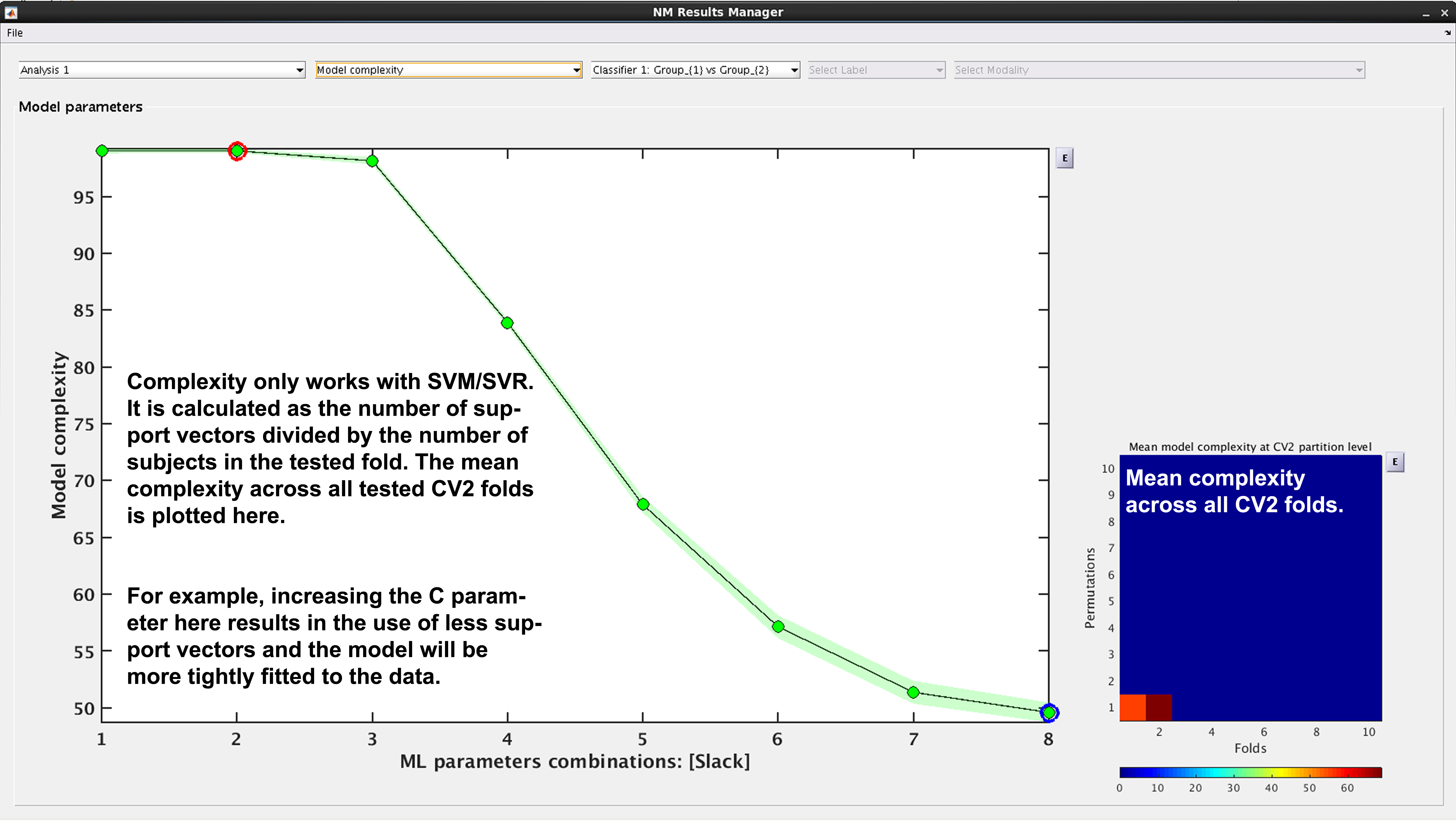
Fig. 17 Result viewer: Model complexity#
Note
Model complexity can only be calculated for LIBSVM and RVM, but not for LIBLINEAR.
Ensemble diversity#
See Fig. 18: This is a measure of Shannon entropy across CV1 models for each CV2 partition. A higher entropy means higher disagreement between the CV1 models. This measure is useful because increased entropy will often result in a better fitting model at the CV2 level. It is useful to note that entropy can be maximized as a performance criterion in addition to accuracy.
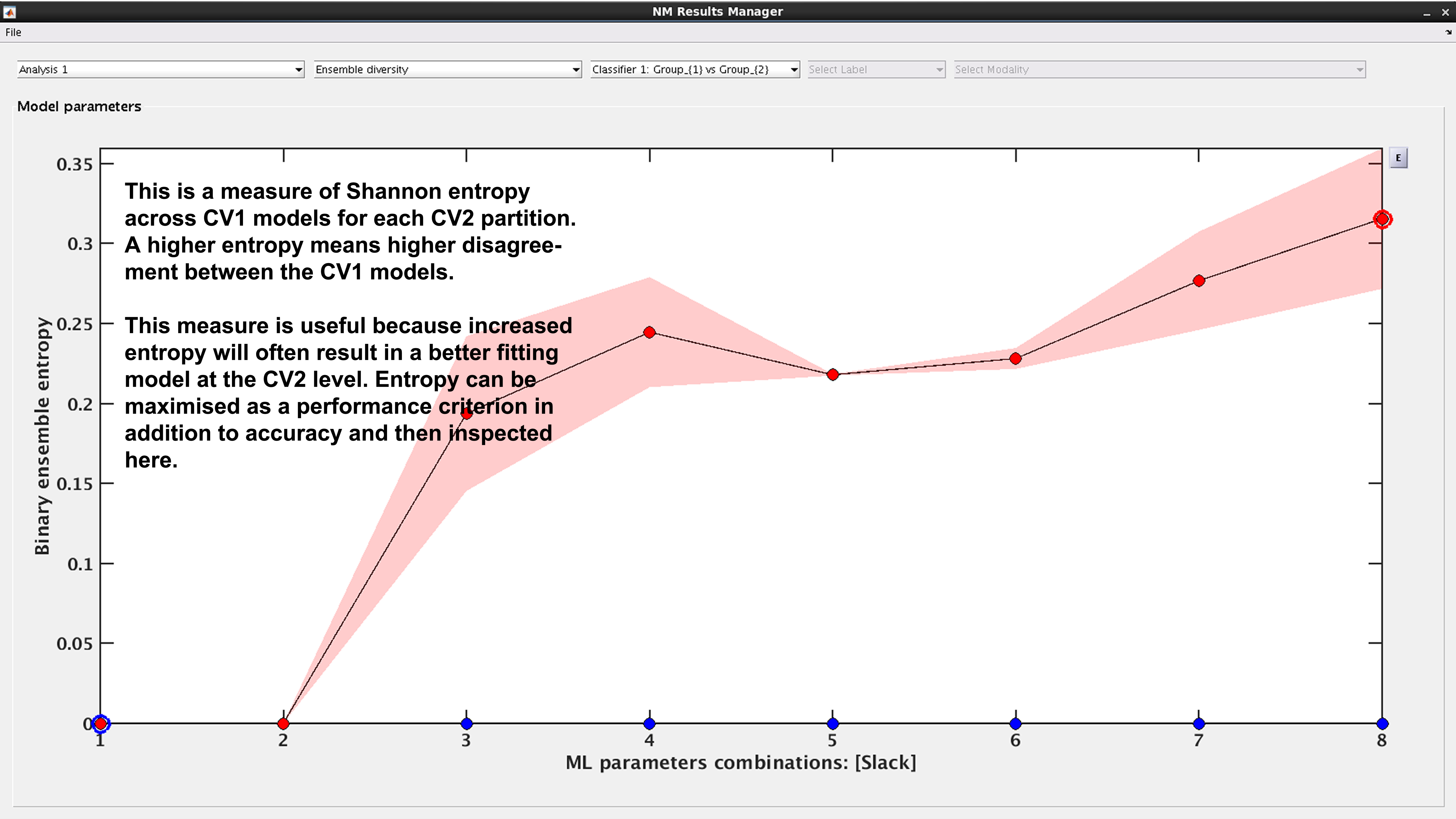
Fig. 18 Result viewer: Ensemble diversity#
Model selection frequency#
See Fig. 19: Within an ensemble framework, the models that are selected within the inner, CV1, cycle are then applied to the outer test data. For example, if it is a 10x10 CV1 framework with a winner-takes-all method of model selection, then 100 models will be applied to the held-out CV2 test fold. This plot displays the percentage of times that each parameter combination was selected.
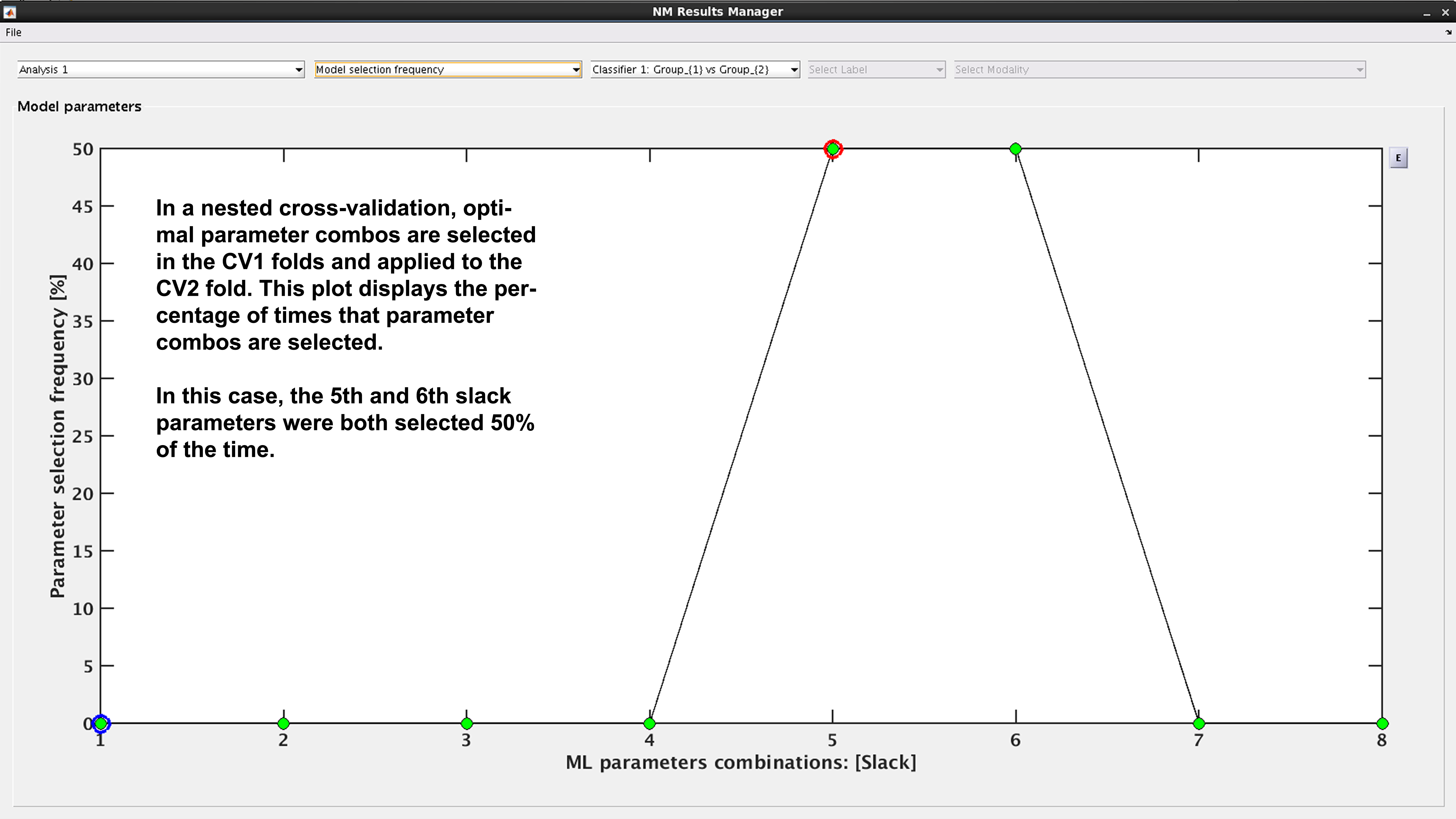
Fig. 19 Result viewer: Model selection frequency#
Multi-group results#
If a multi-group analysis is conducted the results display will change to accommodate the groups. There will be a result section for each classifier and one results section for the multigroup model (see Fig. 20).
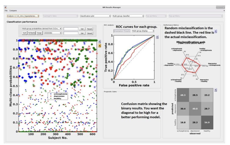
Fig. 20 Result viewer: Multi-group display#
Important
It is important to note that in the misclassification web the red dots are determined by which label (the one above) is misclassified as which label (the one at the bottom). Every corner represents one type of misclassification. The random classification line (the black dashed line) represents the random classification percentage. It differs based on the number of groups in the analysis. For a three-class analysis, it is represented by 6 points at 33%.