Classification algorithm#
Support Vector Machine algorithms are the base of the evaluation core of NeuroMiner. However, a variety of other methods such as k-Nearest Neighbors and Random Forests are also available. In this distribution we rely on the LIBSVM / LIBLINEAR toolboxes for the implementation of support vector based classifiers and regressors. matLearn is also now introduced and requires the Statistics and Optimization Toolbox.
Note
Furthermore, starting with NM 1.1 the MATLAB-Python interface has been implemented and several algorithms from the Scikit-Learn library have been integrated into NM, such as Random Forest and Gradient Boosting. Please see how to install Python for Matlab/NM.
The NeuroMiner interface will change according to the evaluation type selected during data import. Two operation modes are implemented: Classification and Regression. The following will refer to each of these separately.
Classification mode#
In this section we will describe the set up of Classifiers in Neurominer.
Define prediction performance criterion#
During machine learning, models will be optimized and evaluated based on a criterion. For classification problems NeuroMiner provides the following performance measures:
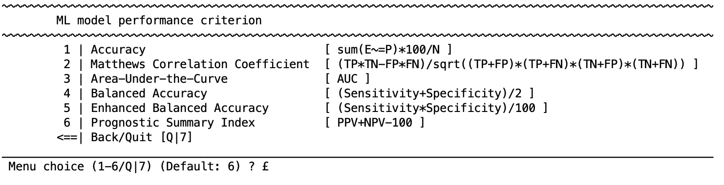
Performance measures
Accuracy (ACC): ACC = sum(E =P)*100/N
True Positive Rate: e.g. for one-class SVM: Sensitivity = TP/(TP+FN)
False Positive Rate: e.g. for one-class SVM: False Positive Rate = FP/(FP+TP)
Positive Predictive Value (PPV): e.g. for one class SVM: PPV = TP/(TP+FP)
Matthews Correlation Coefficient (MCC): MCC = (TP * TN-FP * FN) / sqrt((TP+FP) * (TP+FN) * (TN+FP) * (TN+FN))
Area-Under-the-Curve (AUC): Receiver Operator Characteristic (ROC)
Geometric Mean: Geometric Mean = sqrt(PPV*True Positive Rate)
Balanced Accuracy (BAC): BAC = (sensitivity+specificity) / 2)
[Enhanced Balanced Accuracy]: Enhanced BAC = (sensitivity*specificity)/100)
F-score: F-score = (1+beta2)precisionrecall / (beta2*(precision+recall)) * 100
Prognostic Summary Index: PPV+NPV-100
Number Needed to Predict: 1/PPV
Expected Calibration Error (ECE)
Notes: E: expected, P: predicted, TP: true positive, TN: true negative, FP: false positive, FN: false negative, PPV: positive predictive value, NPV: negative predictive value, ROC: Receiver Operator Characteristic.
Each of these performance measures can have an effect on the resulting model and is dependent on the analysis that is being conducted. For example, simple accuracy is useful when it does not matter if sensitivity and specificity needs to be balanced (e.g., if sensitivity could be very high and specificity very low). However, if there are unequal sample sizes then this can lead to very unbalanced sensitivity and specificity that is an artifact of sample size, which can be corrected by using balanced accuracy (BAC).
Configure learning algorithm#
There are different learning algorithms implemented in NeuroMiner that can be used for classification analyses. Each algorithm has a particular set of parameters that are described in the respective distributions. In general defaults are provided.
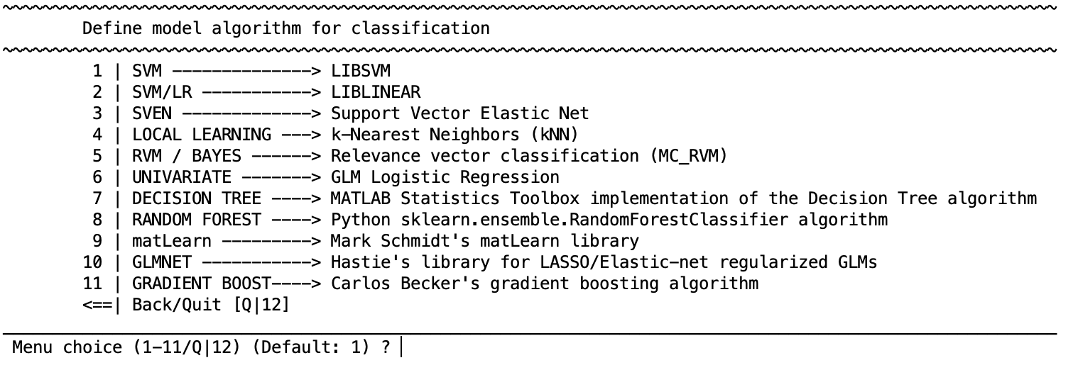
Classification algorithms
SVM - LIBSVM
SVM/LR - LIBLINEAR
SVEN - Support Vector Elastic Net
LOCAL LEARNING - fuzzy k-Nearest Neighbors (kNN )
RVM / BAYES - Relevance vector classification ((ipsorakis/mRVMs))
UNIVARIATE - GLM Logistic Regression (MATLAB glmfit)
DECISION TREE - MATLAB Statistics Toolbox implementation of the Decision Tree algorithm
RANDOM FOREST - Python sklearn.ensemble.RandomForestClassifier algorithm
matLearn - Mark Schmidt’s matLearn library
GLMNET - Hastie’s library for LASSO/Elastic-net regularized GLM(This only works when users have the Statistics and Optimization Toolbox)
GRADIENT BOOST - Python.sklearn.ensemble.GradientBoostingClassifier
ML PERCEPTRON - Python’s sklearn.neural_network.MLPClassifier algorithm
Once one of these option is selected, you will have to define a number of other settings that are specific to the algorithm and can be found in the respective references above. In the following, we present the options that are available for SVM.
Note
When NeuroMiner is opened in expert mode (i.e. by “nm expert”) some additional classification algorithms are available:
NEURAL - Extreme Learning Machine (you have to scale data to -1/1 and prune low-var or NaN vectors)
RVM / BAYES - Psorakis & Damoulas’s implementation with Multiple Kernel Learning
RVM / BAYES - Bayesian Sparse Logistic Regression(for classification in high-D spaces)
LOCAL LEARNING - IMRelief
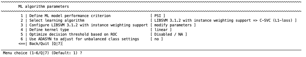
SVM options#
These options depend on the algorithm. For example, the following options will appear when SVM is selected:
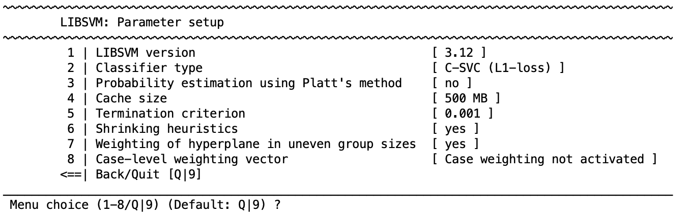
7 | Weight the hyperplane for uneven group sizes
Each of the first 6 options are standard options within the LIBSVM toolbox. However, NeuroMiner also offers hyperplane weighting in uneven group sizes. This is an important option because SVM work effectively when samples are balanced across classes but suboptimal results can emerge when there are unequal class proportions; i.e., the hyperplane can be biased towards a correct classification of the majority class, and thus result in poor classification performance in the minority class. This is called an imbalanced learning problem. To account for this problem a class-weighted SVM can be used. Rather than having equal misclassification penalties (C values) for all individuals this approach corrects for imbalanced learning by increasing the misclassification penalty in the minority class. Specifically, the C parameter for each class is multiplied by the inverse ratio of the training class sizes. To optimize the search for optimal class weights, you can also introduce an additional hyperparameter that multiplies the inverse ratio by a scaling factor for each class prior to the multiplication of the C parameter.
This can be defined when the learning algorithm parameters settings. Similarly, option 8 allows you to weight the hyperplane based on a vector of weighting parameters that you have defined. This will work similarly to the above, but it will use the parameters entered rather than the group sizes.
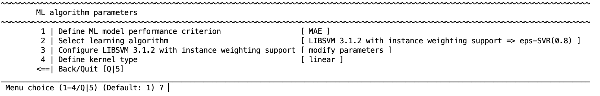
Once these options are selected, NeuroMiner will return to the previous menu where you can also define the kernel type.
Define kernel type#
Define whether the algorithm will use a linear or non-linear kernel Kernel. This will display the following options:
1 | Linear
2 | Polynomial
3 | RBF (Gaussian)
4 | Sigmoid
Once these settings are defined, you will be directed back to the main menu for this section and you can proceed to the main parameter menu where you can configure the learning algorithm).
Regression mode#
If you have defined a regression framework during data input then a different menu will appear as follows.
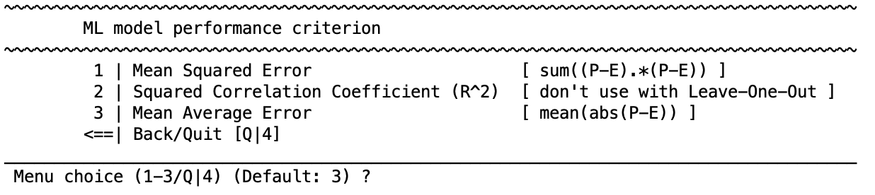
Define prediction performance criterion#
Performance criteria play a major roles in model evaluation and optimization, for regression NM provides 5 performances measures:
Select learning algorithm#
Learning algorithm to be used for the regression analysis. Each algorithm has a particular set of parameters that are described in the respective distributions. In general defaults are provided.
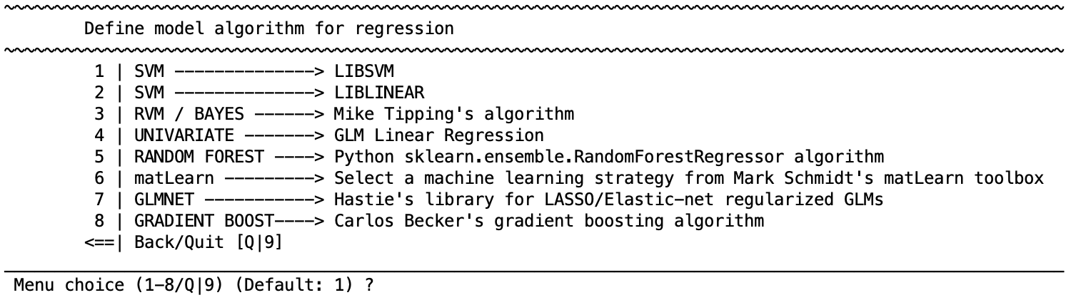
Regression learning algorithms
SVM - LIBSVM
SVM - LIBLINEAR
RVM / BAYES - Mike Tipping’s implementation
Multinomial relevance vector regression (MVRVR) (for multiple target label prediction)
Univariate - GLM Linear Regression
Define kernel type#
Kernel to be used in the selected regressor (when applicable).
Linear
Polynomial
RBF (Gaussian)
Sigmoid
Optimize decision threshold based on ROC (expert mode)#
If you’ve opened NM in expert mode (by calling “nm expert” instead of “nm”), you will have this option (5) in your model setup menu:
It allows optimizing the decision scores according to the Receiver Operator Function. The default setting enables the post-hoc optimization using ROC analysis of C1 test data.
Sequence Optimization#
Note
You need to enter NeuroMiner in EXPERT mode for this (i.e., load NeuroMiner with the command ”nm nosplash expert” or “nm expert”).
When in the NeuroMiner ”expert” mode, another option in the ”model algorithm” menu is to conduct sequence optimization. This option was designed to simulate the clinical decision making associated with additional testing. In a clinical environment, the decision to conduct another assessment on an individual is normally done in situations of uncertainty to confirm a diagnosis – e.g., coronavirus is suspected based on a clinical assessment and then a nasal swab is conducted to confirm this diagnosis. In a machine learning context, uncertainty can be quantified with either the distance from the decision boundary in the case of an SVM (i.e., with cases closer to the decision line being the most uncertain) or with a median using any other scores.
NeuroMiner is able to test sequences of assessments (e.g., clinical, cognitive, imaging) based on the modalities entered during data entry or it is able to build optimal sequences based on different models (e.g., linear and non-linear SVM). The pipelines need to have been analyzed before sequencing can be activated. The procedure is to:
Process multiple analyses as usual from different modalities or using different settings
In the ”Parameter Template” menu, activate the option to 1: Define meta learning/stacking options
Select the analyses that you want to define the optimal sequence for (i.e., in the option “2 | Select 1st-level analyses to provide features to stacker” introduce the indexes of 2 or more analyses you want to stack)
Go to the preprocessing parameters and change the set-up so that there is only an imputation step. If you are sequentially stacking different learning algorithms, then scaling may be required and this needs to be considered
In the ”Parameter Template” menu, go to the ”Classification Algorithm” option and then the ”Select learning algorithm” option
Select the item ”SEQOPT → Predictive sequence optimization algorithm (Stacking only)”
To configure the sequence algorithm, select the option to ”Configure Sequence Optimizer”
You will then see this menu:
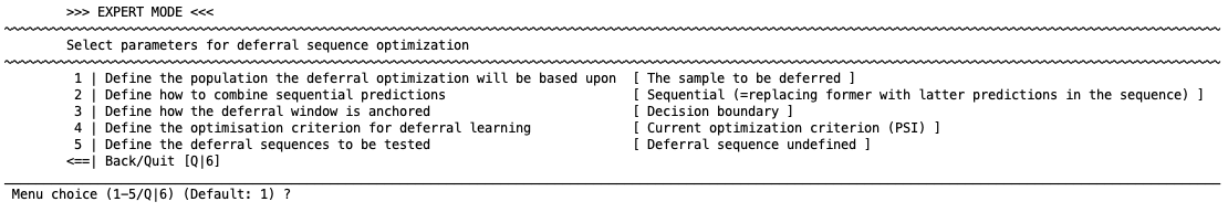
1 | Define the population the deferral optimization will be based on#
1 | The population to be propagated
2 | The entire population
NeuroMiner will attempt to optimize two factors: 1) the criterion that the user decides in the previous step (e.g., BAC); 2) the least number of assessments necessary. These optimizations can be for only the cases that have uncertain decision or probability scores (option 1) or for the entire population.
2 | Define how to combine sequential predictions#
1 | Sequential
2 | Integrative
This option defines the computation mode for combining sequential predictions. When a case is deferred to another model because the first prediction was uncertain, then either its former decision score can be replace with latter predictions in the sequence (“Sequential” computation) or a mean across the predictions in the sequence can be computed (“Integrative” computation, i.e., this becomes bagging or ”late fusion” in NeuroMiner terminology).
3 | Define how the deferral window is anchored#
1 | Decision boundary
2 | Median
As mentioned above, either the decision boundary can be used to define uncertain cases (i.e., near the boundary) or the median of other scores can be taken. The first item uses the decision boundary and the second item uses the median to quantify the uncertainty (i.e., the median of scores that range from very likely group 1 to very likely group 2 is assumed to be uncertain here).
4 | Define optimization criterion fro deferral learning#
1 | Current optimization criterion
2 | Mean decision distance
Here the user can select whether to optimize the criterion previously selected (e.g., the BAC) or the mean decision distance (only works for algorithms which output decision scores/probabilities). In the second case, the underlying idea is that the optimization is better the further away the score is from the decision boundary.
5 | Sequences to be tested#
1 | Define sequences matrix to be evaluated
Here the user can define what sequences are to be evaluated. This step is dependent on the identification of models to be included in the ”1: Define meta learning/stacking options”. The idea is that rather than testing all combinations of the models (e.g., model 1 - model 2 - model 3 and then all other combinations of these), the user can specify the models that they want to test. This is because usually there is a rationale for testing model sequences based on clinical experience and also cost (e.g., clinical assessment, then cognitive assessment, then imaging if necessary).
Sequences of assessments need to be specified here either directly or using a MATLAB variable. For example, if you wanted to specify a sequence of model 1 - model 2 - model 3 then you would enter [1 2 3]. If you wanted to specify this and also models 2 1 3 then you would enter [1 2 3; 2 1 3]. If you want to specify more, you can create a MATLAB variable with more sequences in rows and you can enter the variable name into this section.You can also combine sequences with different numbers of examinations. Use Nan padding to fill the missing examination in shorter sequences, e.g. by entering [1 NaN NaN; 2 1 NaN; 3 2 1]. We recommend predefining the sequences in a spreadsheet program and then pasting them into a MATLAB variable at the command line. The variable can then be entered at the menu prompt by typing its name.
Afterwards you can return to the main menu, initialize your analyses and train as indicated in stacking.
Note
Sequence optimization is currently only available in classification mode.